Calibration of carbon back to almost 50, years ago has been done in several ways. One way is to find yearly layers that are produced over longer periods of time than tree rings. In some lakes or bays where underwater sedimentation occurs at a relatively rapid rate, the sediments have seasonal patterns, so each year produces a distinct layer. Such sediment layers are called "varves", and are described in more detail below.

Varve layers can be counted just like tree rings.

Radiometric Dating

If layers contain dead plant material, they can be used to calibrate the carbon ages. Another way to calibrate carbon farther back in time is to find recently-formed carbonate deposits and cross-calibrate the carbon in them with another short-lived radioactive isotope. Where do we find recently-formed carbonate deposits?

If you have ever taken a tour of a cave and seen water dripping from stalactites on the ceiling to stalagmites on the floor of the cave, you have seen carbonate deposits being formed. Since most cave formations have formed relatively recently, formations such as stalactites and stalagmites have been quite useful in cross-calibrating the carbon record. What does one find in the calibration of carbon against actual ages? If one predicts a carbon age assuming that the ratio of carbon to carbon in the air has stayed constant, there is a slight error because this ratio has changed slightly.

Figure 9 shows that the carbon fraction in the air has decreased over the last 40, years by about a factor of two. This is attributed to a strengthening of the Earth's magnetic field during this time. A stronger magnetic field shields the upper atmosphere better from charged cosmic rays, resulting in less carbon production now than in the past. Changes in the Earth's magnetic field are well documented.

Complete reversals of the north and south magnetic poles have occurred many times over geologic history. A small amount of data beyond 40, years not shown in Fig. What change does this have on uncalibrated carbon ages? The bottom panel of Figure 9 shows the amount. Ratio of atmospheric carbon to carbon, relative to the present-day value top panel.

Evaluation and presentation schemes in dating

Tree-ring data are from Stuiver et al. The offset is generally less than years over the last 10, years, but grows to about 6, years at 40, years before present. Uncalibrated radiocarbon ages underestimate the actual ages.

1. Navigation menu;
2. what are the most popular dating sites in australia.
3. atomic dating.
4. over 30 singles dating.
5. only see the guy im dating once a week.
6. Radioactive dating - The Australian Museum?
7. Dating Methods Using Radioactive Isotopes?

Note that a factor of two difference in the atmospheric carbon ratio, as shown in the top panel of Figure 9, does not translate to a factor of two offset in the age. Rather, the offset is equal to one half-life, or 5, years for carbon The initial portion of the calibration curve in Figure 9 has been widely available and well accepted for some time, so reported radiocarbon dates for ages up to 11, years generally give the calibrated ages unless otherwise stated.

The calibration curve over the portions extending to 40, years is relatively recent, but should become widely adopted as well. It is sometimes possible to date geologically young samples using some of the long-lived methods described above. These methods may work on young samples, for example, if there is a relatively high concentration of the parent isotope in the sample.

In that case, sufficient daughter isotope amounts are produced in a relatively short time. As an example, an article in Science magazine vol. There are other ways to date some geologically young samples. Besides the cosmogenic radionuclides discussed above, there is one other class of short-lived radionuclides on Earth. These are ones produced by decay of the long-lived radionuclides given in the upper part of Table 1.

Radiometric dating

As mentioned in the Uranium-Lead section, uranium does not decay immediately to a stable isotope, but decays through a number of shorter-lived radioisotopes until it ends up as lead. While the uranium-lead system can measure intervals in the millions of years generally without problems from the intermediate isotopes, those intermediate isotopes with the longest half-lives span long enough time intervals for dating events less than several hundred thousand years ago. Note that these intervals are well under a tenth of a percent of the half-lives of the long-lived parent uranium and thorium isotopes discussed earlier.

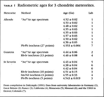
Two of the most frequently-used of these "uranium-series" systems are uranium and thorium These are listed as the last two entries in Table 1, and are illustrated in Figure A schematic representation of the uranium decay chain, showing the longest-lived nuclides.

Half-lives are given in each box. Solid arrows represent direct decay, while dashed arrows indicate that there are one or more intermediate decays, with the longest intervening half-life given below the arrow. Like carbon, the shorter-lived uranium-series isotopes are constantly being replenished, in this case, by decaying uranium supplied to the Earth during its original creation. Following the example of carbon, you may guess that one way to use these isotopes for dating is to remove them from their source of replenishment.

This starts the dating clock. In carbon this happens when a living thing like a tree dies and no longer takes in carbonladen CO 2. For the shorter-lived uranium-series radionuclides, there needs to be a physical removal from uranium. The chemistry of uranium and thorium are such that they are in fact easily removed from each other.

Uranium tends to stay dissolved in water, but thorium is insoluble in water. So a number of applications of the thorium method are based on this chemical partition between uranium and thorium. Sediments at the bottom of the ocean have very little uranium relative to the thorium. Because of this, the uranium, and its contribution to the thorium abundance, can in many cases be ignored in sediments. Thorium then behaves similarly to the long-lived parent isotopes we discussed earlier. It acts like a simple parent-daughter system, and it can be used to date sediments. On the other hand, calcium carbonates produced biologically such as in corals, shells, teeth, and bones take in small amounts of uranium, but essentially no thorium because of its much lower concentrations in the water.

This allows the dating of these materials by their lack of thorium. A brand-new coral reef will have essentially no thorium As it ages, some of its uranium decays to thorium While the thorium itself is radioactive, this can be corrected for. Comparison of uranium ages with ages obtained by counting annual growth bands of corals proves that the technique is.

The method has also been used to date stalactites and stalagmites from caves, already mentioned in connection with long-term calibration of the radiocarbon method. In fact, tens of thousands of uranium-series dates have been performed on cave formations around the world. Previously, dating of anthropology sites had to rely on dating of geologic layers above and below the artifacts. But with improvements in this method, it is becoming possible to date the human and animal remains themselves.

Work to date shows that dating of tooth enamel can be quite reliable. However, dating of bones can be more problematic, as bones are more susceptible to contamination by the surrounding soils. As with all dating, the agreement of two or more methods is highly recommended for confirmation of a measurement. If the samples are beyond the range of radiocarbon e. We will digress briefly from radiometric dating to talk about other dating techniques. It is important to understand that a very large number of accurate dates covering the past , years has been obtained from many other methods besides radiometric dating.

We have already mentioned dendrochronology tree ring dating above. Dendrochronology is only the tip of the iceberg in terms of non-radiometric dating methods. Here we will look briefly at some other non-radiometric dating techniques. One of the best ways to measure farther back in time than tree rings is by using the seasonal variations in polar ice from Greenland and Antarctica. There are a number of differences between snow layers made in winter and those made in spring, summer, and fall.

These seasonal layers can be counted just like tree rings. The seasonal differences consist of a visual differences caused by increased bubbles and larger crystal size from summer ice compared to winter ice, b dust layers deposited each summer, c nitric acid concentrations, measured by electrical conductivity of the ice, d chemistry of contaminants in the ice, and e seasonal variations in the relative amounts of heavy hydrogen deuterium and heavy oxygen oxygen in the ice.

These isotope ratios are sensitive to the temperature at the time they fell as snow from the clouds. The heavy isotope is lower in abundance during the colder winter snows than it is in snow falling in spring and summer. So the yearly layers of ice can be tracked by each of these five different indicators, similar to growth rings on trees. The different types of layers are summarized in Table III. Ice cores are obtained by drilling very deep holes in the ice caps on Greenland and Antarctica with specialized drilling rigs.

As the rigs drill down, the drill bits cut around a portion of the ice, capturing a long undisturbed "core" in the process. These cores are carefully brought back to the surface in sections, where they are catalogued, and taken to research laboratories under refrigeration. A very large amount of work has been done on several deep ice cores up to 9, feet in depth.

Several hundred thousand measurements are sometimes made for a single technique on a single ice core. A continuous count of layers exists back as far as , years.

In addition to yearly layering, individual strong events such as large-scale volcanic eruptions can be observed and correlated between ice cores. A number of historical eruptions as far back as Vesuvius nearly 2, years ago serve as benchmarks with which to determine the accuracy of the yearly layers as far down as around meters.

Radioactive dating

As one goes further down in the ice core, the ice becomes more compacted than near the surface, and individual yearly layers are slightly more difficult to observe. For this reason, there is some uncertainty as one goes back towards , years. Recently, absolute ages have been determined to 75, years for at least one location using cosmogenic radionuclides chlorine and beryllium G. These agree with the ice flow models and the yearly layer counts. Note that there is no indication anywhere that these ice caps were ever covered by a large body of water, as some people with young-Earth views would expect.

Polar ice core layers, counting back yearly layers, consist of the following:. Visual Layers Summer ice has more bubbles and larger crystal sizes Observed to 60, years ago Dust Layers Measured by laser light scattering; most dust is deposited during spring and summer Observed to , years ago Layering of Elec-trical Conductivity Nitric acid from the stratosphere is deposited in the springtime, and causes a yearly layer in electrical conductivity measurement Observed through 60, years ago Contaminant Chemistry Layers Soot from summer forest fires, chemistry of dust, occasional volcanic ash Observed through 2, years; some older eruptions noted Hydrogen and Oxygen Isotope Layering Indicates temperature of precipitation.

Heavy isotopes oxygen and deuterium are depleted more in winter. Yearly layers observed through 1, years; Trends observed much farther back in time Varves. Another layering technique uses seasonal variations in sedimentary layers deposited underwater. The two requirements for varves to be useful in dating are 1 that sediments vary in character through the seasons to produce a visible yearly pattern, and 2 that the lake bottom not be disturbed after the layers are deposited.

These conditions are most often met in small, relatively deep lakes at mid to high latitudes.